Driver2Vec

Reproduction of Driver2Vec paper by Yang et al. (2021).

Authors: Danish Khan, Achille Bailly and Mingjia He

Introduction

The neural network architecture Driver2Vec is discussed and used to detect drivers from automotive data in this blogpost. Yang et al. published a paper in 2021 that explained and evaluated Driver2Vec, which outperformed other architectures at that time. Driver2Vec (is the first architecture that) blends temporal convolution with triplet loss using time series data [1]. With this embedding, it is possible to classify different driving styles. The purpose of this reproducibility project is to recreate the Driver2Vec architecture and reproduce Table 5 from the original paper. The purpose of this blog post is to give a full explanation of this architecture as well as to develop it from the ground up.

Researchers employ sensors found in modern vehicles to determine distinct driving patterns. In this manner, the efficacy is not dependent on invasive data, such as facial recognition or fingerprints. A system like this may detect who is driving the car and alter its vehicle settings accordingly. Furthermore, a system that recognizes driver types with high accuracy may be used to identify unfamiliar driving patterns, lowering the chance of theft.

Method

Driver2Vec transforms a 10-second clip of sensor data to an embedding that is being used to identify different driving styles [1]. This procedure can be broken down into two steps. In the first stage, a temporal convolutional network (TCN) and a Haar wavelet transform are utilized individually, then concatenated to generate a 62-length embedding. This embedding is intended such that drivers with similar driving styles are near to one another while drivers with different driving styles are further apart.

Temporal Convolutional Network (TCN)

Temporal Convolutional Networks (TCN) combines the architecture of convolutional networks and recurrent networks. The principle of TCN consists of two aspects:

1. The output of TCN has the same length as the input.
2. TCN uses causal convolutions, where an output at a specific time step is only depend on the input from this time step and earlier in the previous layer.

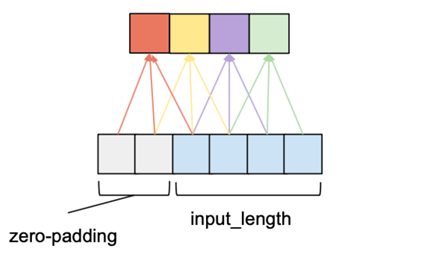
To ensure the first principle, zero padding is applied. As shown in Figure 1, the zero padding is applied on the left side of the input tensor and ensure causal convolution. In this case, the kernel size is 3 and the input length is 4. With a padding size of 2, the output length is equal to the input length.

Figure 1. Zero padding [2]

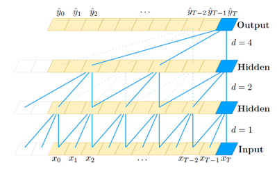
One of the problems of casual convolution is that the history size it can cover is linear in the depth of network. Simple casual convolution could be challenging when dealing with sequential tasks that require a long history coverage, as very deep network would have many parameters, which may expand training time and lead to overfitting. Thus, dilated convolution is used to increase the receptive field size while having a small number of layers. Dilation is the name for the interval length between the elements in a layer used to compute one element of the next layer. The convolution with a dilation of one is a simple regular convolution. In TCN, dilation exponentially increases as progress through the layers. As shown in Figure 2, as the network moves deeper, the elements in the next layer cover larger range of elements in the previous layer.

Figure 2. An example of dilated causal convolution [3]

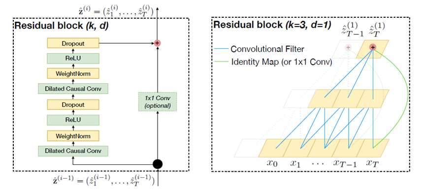
TCN employs generic residual module in place of a convolutional layer. The structure of residual connection is shown in Figure 3, in each residual block, TCN has two layers including dilated causal convolution, weight normalization, rectified linear unit (ReLU) and dropout.

Figure 3. The residual module in TCN [3]

Haar Wavelet Transform

Driver2vec applied Haar wavelet transformation to generates two vectors in the frequency domain. Wavelet Transform decomposes a time series function into a set of wavelets. A Wavelet is an oscillation use to decompose the signal, which has two characteristics, scale and location. Large scale can capture low frequency information and conversely, small scale is designed for high frequency information. Location defines the time and space of the wavelet.

The essence of Wavelet Transform is to measure how much of a wavelet is in a signal for a particular scale and location. The process of Wavelet Transform consists of four steps:

1. the wavelet moves across the entire signal with various location
2. the coefficients of trend and fluctuation for at each time step is calculated use scalar product (in following equations)
3. increase the wavelet scale
4. repeat the process.

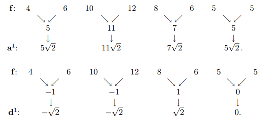
Most specifically, the Haar transform decomposes a discrete signal into two sub-signals of half its length, one is a running average or trend and the other is a running difference or fluctuation. As shown in the following equations, the first trend subsignal is computed from the average of two values and fluctuation, the second trend subsignal, is computed by taking a running difference, as shown in Equation 2. This structure enable transform to detect small fluctuations feature in signals. Figure 4 shows how Haar transform derives sub-signals for the signal \(f=(4, 6, 10, 12, 8, 6, 5, 5)\)

Figure 4. An example for Haar transform [4]

Full architecture

The two vectors that the wavelet transform outputs are then fed through a Fully Connected (FC) layer to map them to a 15 dimensional vector. Both of them are concatenated with the last output of the TCN and fed through a final FC layer with Batch Normalization and a sigmoid activation function to get our final embedding.

Triplet Margin Loss

Once we the embedding from the full architecture, we need a way to train the network. With no ground truth to compare the output to, the triplet margin loss is used. At its core, this criterion pulls together the embeddings that are supposed to be close and pushes away the ones that are not. Mathematically, it is defined as follows:

Where \(x_r, x_p, x_n\) are the embeddings for the anchor, positive and negative samples respectively, \(D_{rp}\) (resp. \(D_{rn}\)) is the distance (usually euclidean) between the anchor and the positive embeddings (resp. negative) and \(\alpha\) is a positive number called the margin (often set to \(1.0\)).

Essentially, it is trying to make sure that the following inequality is respected:

With the available dataset being so limited, choosing the positive and negative samples for each anchor at random is probably enough. In most cases however, the most efficient way of choosing them is to pick the worst ones for each anchor (see [5]), i.e. choosing the positive sample that is the farthest away and the negative one that is the closest. Again, for more detail on how to actually do that efficiently, go to the website referenced in [5] for a very detailed explanation.

In the end, we chose to implement the "hard" triplet loss as we thought it might resolve the issues we faced.

Gradient Boosting Decision Trees (LightGBM)

Before introducing Light GBM, we first illustrate what is boosting and how it can work. The goal of boosting is improving the prediction power converting weak learners into strong learners. The basic logit is to build a model on the training dataset, and then build the next model to rectify the errors present in the previous one. In this procedure, weights of observations are updates according to the rule that wrongly classified observations would have increasing weights. So, only those misclassified observations get selected in the next model and the procedure iterate until the errors are minimized.

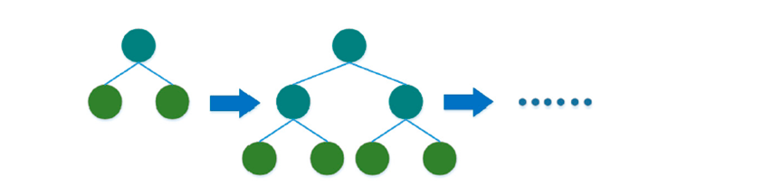
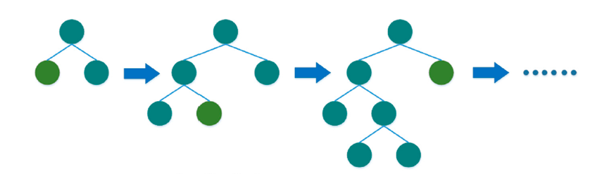
Gradient Boosting trains many models in an additive and sequential manner, using gradient decent to minimize the loss function One of the most popular types of gradient boosting is boosted decision trees. There are two different strategies to compute the trees: level-wise and leaf-wise, as shown in the following figure. The level-wise strategy grows the tree level by level. In this strategy, each node splits the data prioritizing the nodes closer to the tree root. The leaf-wise strategy grows the tree by splitting the data at the nodes with the highest loss change.

Figure 5. The level-wise strategy [6]

Figure 6. The leaf-wise strategy [6]

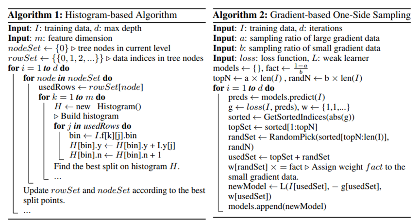
However, conventional gradient decision tree could be inefficient when dealing with large scale data set. That is why Light GBM is proposed, which is a gradient boosting decision tree with Gradient-based One-Side Sampling (GOSS) and Exclusive Feature Bundling (EFB). Light GBM is based on tree-based learning algorithms growing tree vertically (leaf-wise). It is designed to be distributed and efficient with the following advantages [7]:

• Faster training speed and higher efficiency.

• Lower memory usage.

• Better accuracy.

• Support of parallel, distributed, and GPU learning.

• Capable of handling large-scale data.

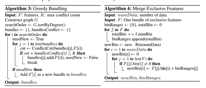
GOSS is a design for the sampling process with the aim to reduce computation cost and not lose much training accuracy. The instances with large gradients would be better kept considering those bearing more information gain, and the instances with small gradients will be randomly drop. EFB tries to effectively reduce the number of features in a nearly lossless manner. A feature scanning algorithm is designed to build feature histograms from the feature bundles. The algorithms used in presented in the following figures (refer to the work of Ke. G et al. [8]).

Figure 7. Algorithms for Light GBM [8]

Light GBM has been widely used due to its ability to handle the large size of data and takes lower memory to run. But it should be noted that there are shortcomings: Light GBM is sensitive to overfitting and can easily overfit small data.

Data

The original dataset includes 51 anonymous driver test drives on four distinct types of roads (highway, suburban, urban, and tutorial), with each driver spending roughly fifteen minutes on a high-end driving simulator built by Nervtech [1]. However, this entire dataset is not made publicly available and instead, only a small sample of the dataset can be found in a anonymized repository on Github. Instead of 51 drivers and fifteen minutes of recording time, this sample has ten second samples captured at 100Hz of five drivers for each distinct road type. As a result, the sample size is dramatically reduced.

Nine groups

The columns remain identical. Although both the original and sampled datasets include 38 columns, only 31 of them are used for the architecture, which is divided into nine categories.

1. Acceleration

Column names	Description
ACCELERATION	acceleration in X axis
ACCELERATION_Y	acceleration in Y axis
ACCELERATION_Z	acceleration in Z axis

2. Distance information

Column names	Description
DISTANCE_TO_NEXT_VEHICLE	distance to next vehicle
DISTANCE_TO_NEXT_INTERSECTION	distance to next intersection
DISTANCE_TO_NEXT_STOP_SIGNAL	distance to next stop signal
DISTANCE_TO_NEXT_TRAFFIC_LIGHT_SIGNAL	distance to next traffic light
DISTANCE_TO_NEXT_YIELD_SIGNAL	distance to next yield signal
DISTANCE	distance to completion

3. Gearbox

Column names	Description
GEARBOX	whether gearbox is used
CLUTCH_PEDAL	whether clutch pedal is pressed

4. Lane Information

Column names	Description
LANE	lane that the vehicle is in
FAST_LANE	whether vehicle is in the fast lane
LANE_LATERAL_SHIFT_RIGHT	location in lane (right)
LANE_LATERAL_SHIFT_CENTER	location in lane (center)
LANE_LATERAL_SHIFT_LEFT	location in lane (left)
LANE_WIDTH	width of lane

5. Pedals

Column names	Description
ACCELERATION_PEDAL	whether acceleration pedal is pressed
BRAKE_PEDAL	whether break pedal is pressed

6. Road Angle

Column names	Description
STEERING_WHEEL	angle of steering wheel
CURVE_RADIUS	radius of road (if there is a curve)
ROAD_ANGLE	angle of road

7. Speed

Column names	Description
SPEED	speed in X axis
SPEED_Y	speed in Y axis
SPEED_Z	speed in Z axis
SPEED_NEXT_VEHICLE	speed of the next vehicle
SPEED_LIMIT	speed limit of road

8. Turn indicators

Column names	Description
INDICATORS	whether turn indicator is on
INDICATORS_ON_INTERSECTION	whether turn indicator is activated for an intersection

9. Uncategorized

Column names	Description
HORN	whether horn is activated
HEADING	heading of vehicle

(10. Omitted from Driver2Vec)

Column names	Description
FOG	whether there is fog
FOG_LIGHTS	whether fog light is on
FRONT_WIPERS	whether front wiper is activated
HEAD_LIGHTS	whether headlights are used
RAIN	whether there is rain
REAR_WIPERS	whether rear wiper is activated
SNOW	whether there is snow

Results

After reconstructing the Driver2Vec architecture, we let this model train on the sampled data. The performance is assessed by looking at the pairwise accuracy. This means that we are now in a binary classification setting, where the model does a prediction on every possible pair among all five drivers. The average accuracy is then reported. Moreover, the (average) pairwise accuracy is computed after having each sensor group removed from the data. This way the ablation study on Driver2Vec (Table 5 from original paper) is redone.

Removed Sensor Group	Original Pairwise Accuracy (%)	Pairwise Accuracy (%)
Speed, acceleration only	66.3	66.7
Distance information	74.6	65.7
Lane information	77.8	68.3
Acceleration/break pedal	78.1	69.5
Speed	78.8	65.3
Gear box	79.0	56.5
Acceleration	79.1	66.7
Steering wheel/road angle	79.2	69.7
Turn indicators	79.3	64.7
All Sensor Groups included	81.8	71.5

Based on the results found in this table, and with the limited data at hand, the reproduced architecture shows signs of identifying different driving styles. However, all reproduced results are lower compared to the original accuracies.

Aside from the lack of data, the decrease in accuracy could be caused by the Triplet Margin Loss function. Throughout the experiments, we saw that the loss kept converging to the margin, rather than decreasing to zero. From this, we interpret that it is much more difficult to find an embedding that satisfies the inequality \(D_{rp}^{2} + \alpha < D_{rp}^{2}\). This might be due to the way the architecture was implemented.

Reference

[1] Yang, J., Zhao, R., Zhu, M., Hallac, D., Sodnik, J., & Leskovec, J. (2021). Driver2vec: Driver identification from automotive data. arXiv preprint arXiv:2102.05234.

[2] Francesco, L. (2021). Temporal Convolutional Networks and Forecasting. https://unit8.com/resources/temporal-convolutional-networks-and-forecasting/

[3] Bai, S., Kolter, J. Z., & Koltun, V. (2018). An empirical evaluation of generic convolutional and recurrent networks for sequence modeling. arXiv preprint arXiv:1803.01271.

[4] Haar Wavelets http://dsp-book.narod.ru/PWSA/8276_01.pdf

[5] Good explanation and implementation (in Tensorflow) of the Triplet Loss: https://omoindrot.github.io/triplet-loss

[6] What is LightGBM https://medium.com/@pushkarmandot/https-medium-com-pushkarmandot-what-is-lightgbm-how-to-implement-it-how-to-fine-tune-the-parameters-60347819b7fc

[7] LightGBM’s documentation, Microsoft Corporation https://lightgbm.readthedocs.io/en/latest/

[8] Ke, G., Meng, Q., Finley, T., Wang, T., Chen, W., Ma, W., ... & Liu, T. Y. (2017). Lightgbm: A highly efficient gradient boosting decision tree. Advances in neural information processing systems, 30.